Maps
Data Visualization, Week 5
Kieran Healy, Duke University
Outline for Today
- Housekeeping
- Reviewing the Homework
- Git
- Maps
How to Navigate these Slides
- When you view them online, notice the compass in the bottom right corner
- You can go left or right, or sometimes down to more detail.
- Hit the
Escapekey to get an overview of all the slides. On a phone or tablet, pinch to get the slide overview. - You can use the arrow keys (or swipe up and down) in this view, as well.
- Hit
Escapeagain to return to the slide you were looking at. - On a phone or tablet, tap the slide you want.
Git
Git is Horrible
- But it can help you keep track of what you did
- It's also where a lot of software development happens
- So it's worth getting a feel for it
Simplest GitHub Use Case
- You have no account there.
- You download stuff from it.
Next Simplest GitHub Use Case
- You have an account there.
- You fork (i.e., copy) things on other people's GitHub accounts to your GitHub account.
- Then you clone (i.e., copy, or download) them to your laptop.
- This kind of confusing, doubled-up, garbage terminology is typical of Git.
Basic One-Person Regular Git Use Case
- You have a file under version control.
- You make a change to it and save the file.
- You stage or
adda snapshot of the changed files, - Then you
committhe snapshot of changes to the repository, with a message saying what you did.
Basic One-Person Regular Git Use Case
- You have a file under version control.
- You make a change to it and save the file.
- You stage or
adda snapshot of the changed files, - Then you
committhe snapshot of changes to the repository, with a message saying what you did. - You
pushthat change up to e.g. GitHub.
Tutorial
Data Manipulation
Maps
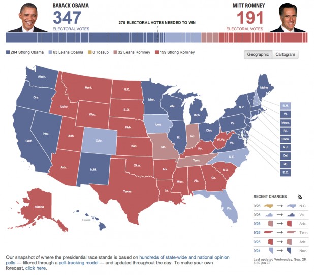
2012 US Election, Winner by State
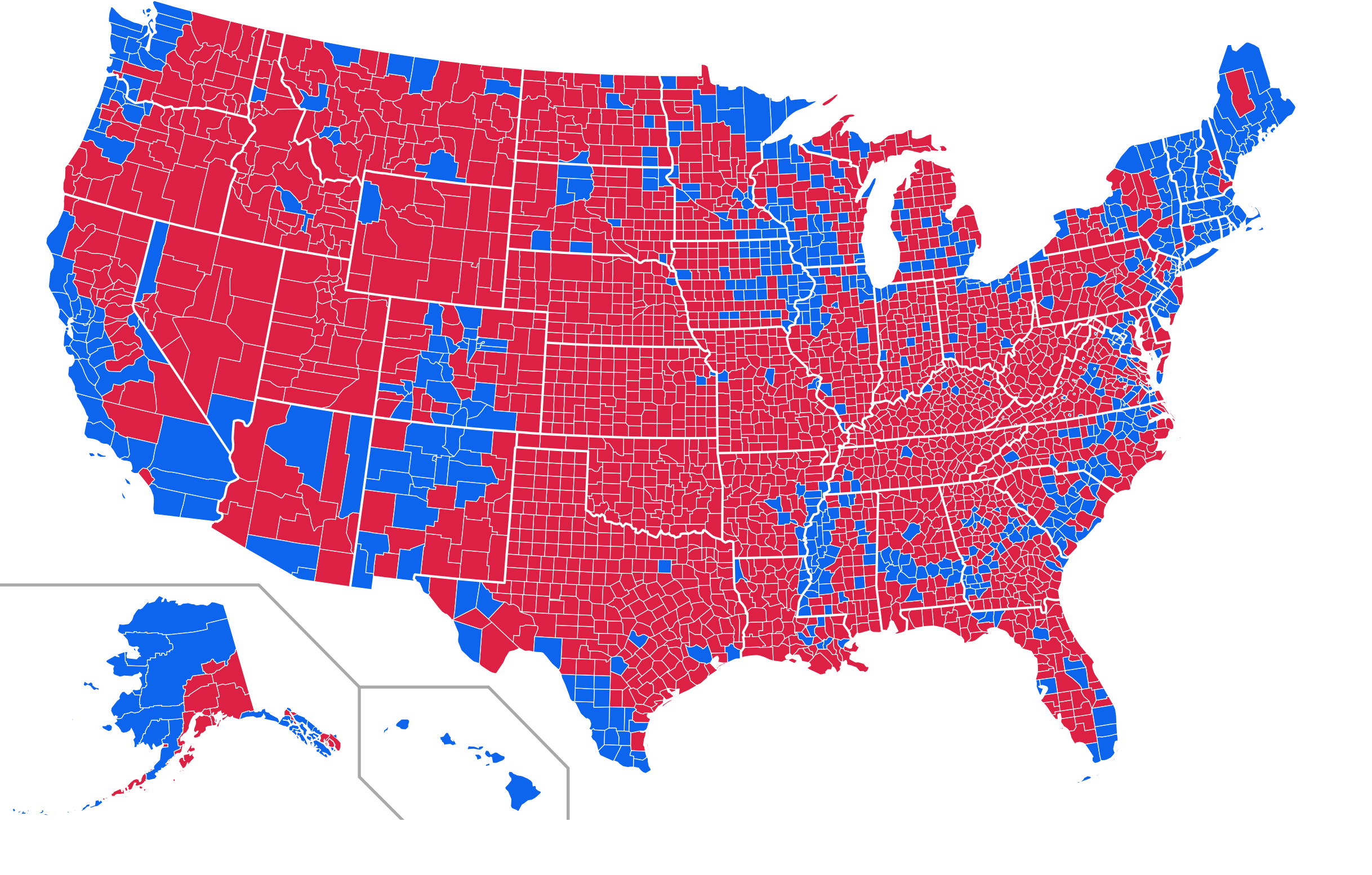
2012 US Election, Winner by County
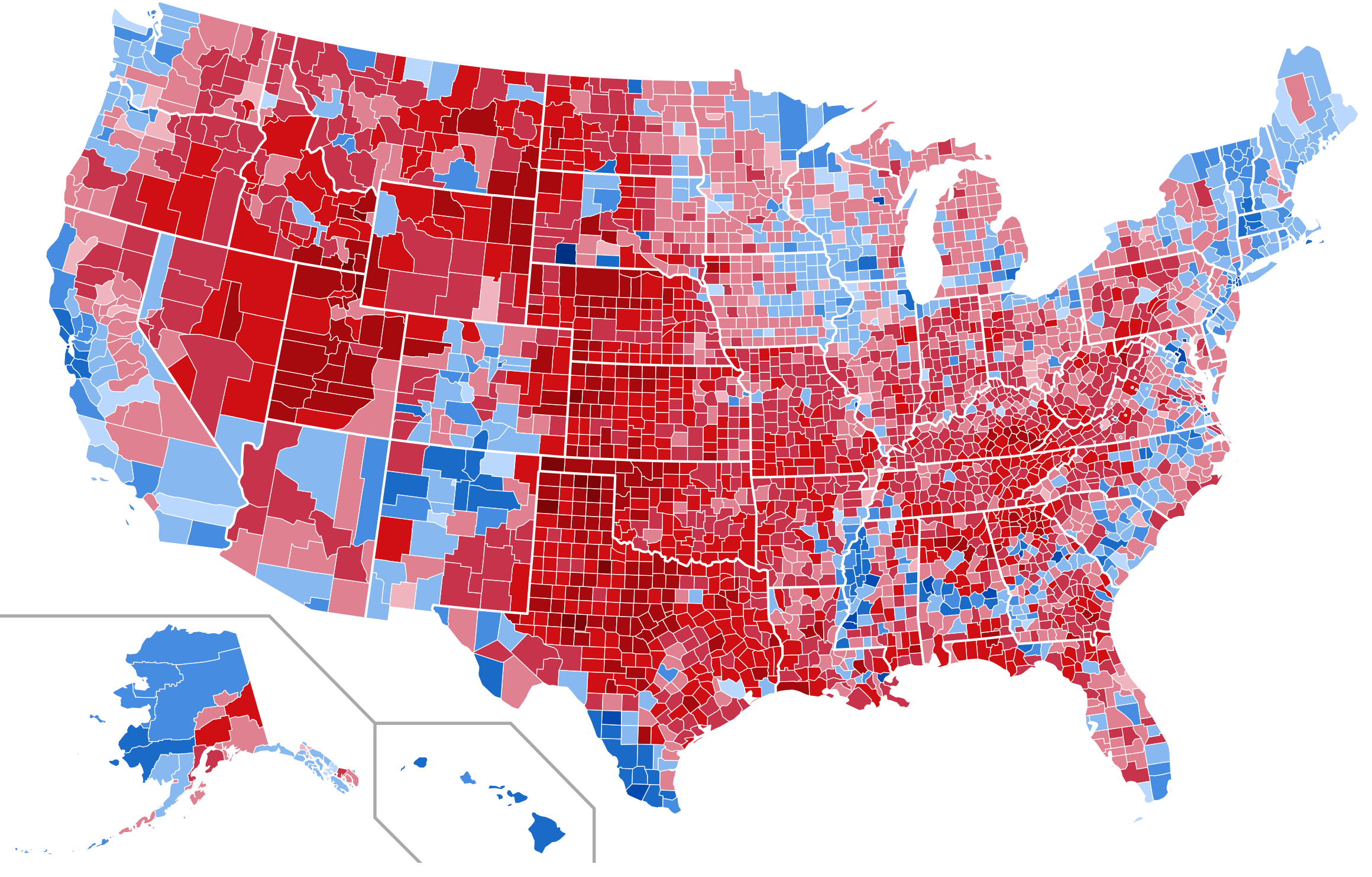
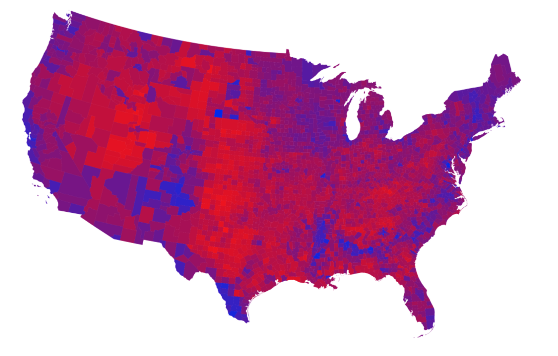
2012 US Election, Winner by County Share
2012 US Election, Color-Centered
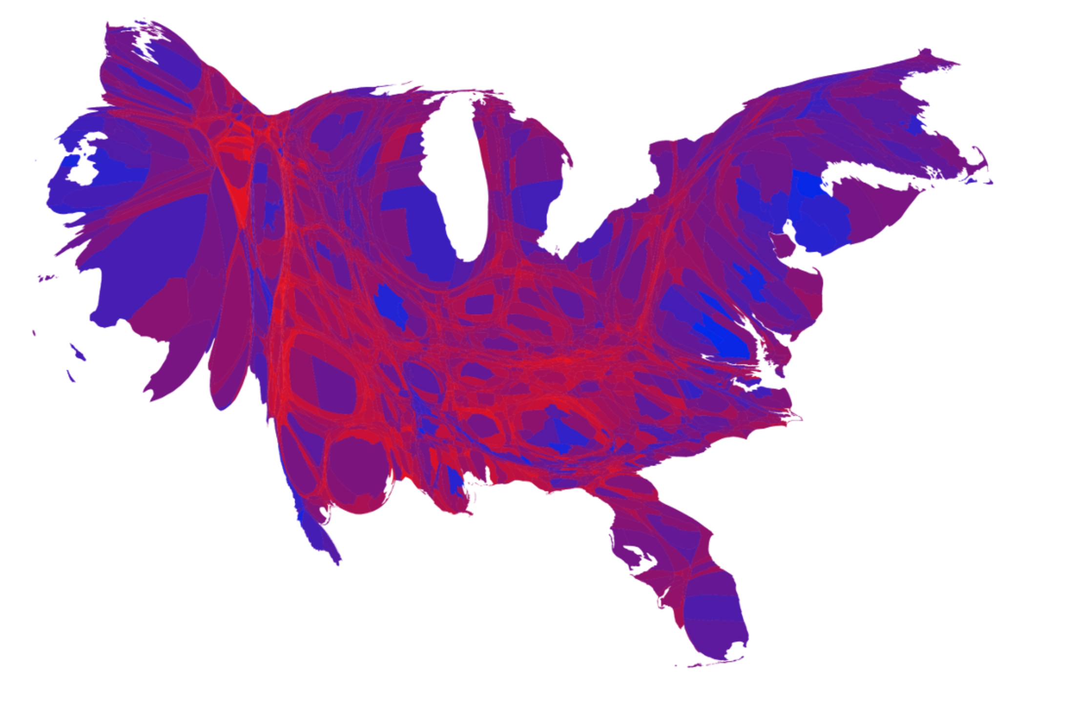
2012 US Election, Color-Centered, Scaled by Population
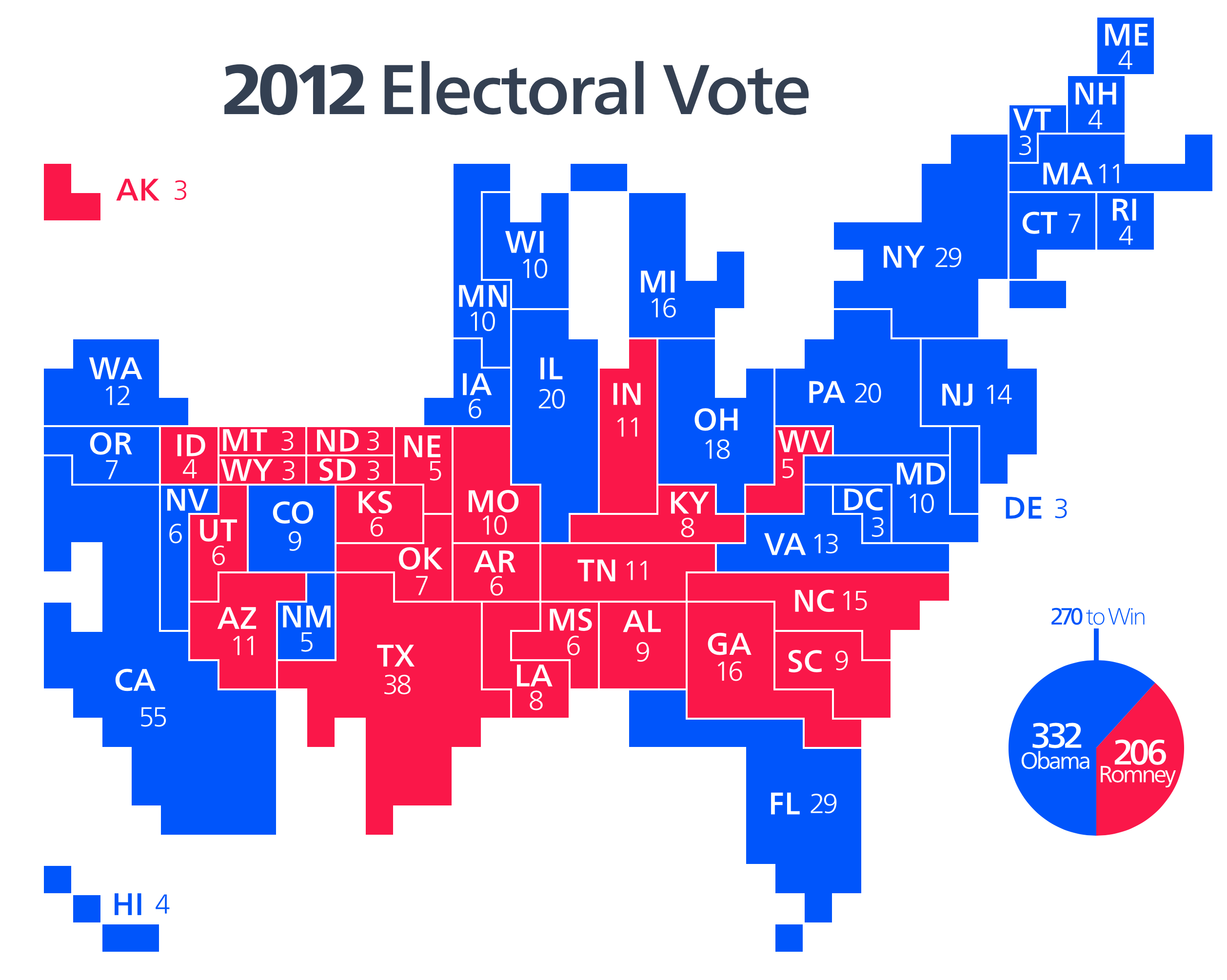
2012 US Election, Electoral College Cartogram
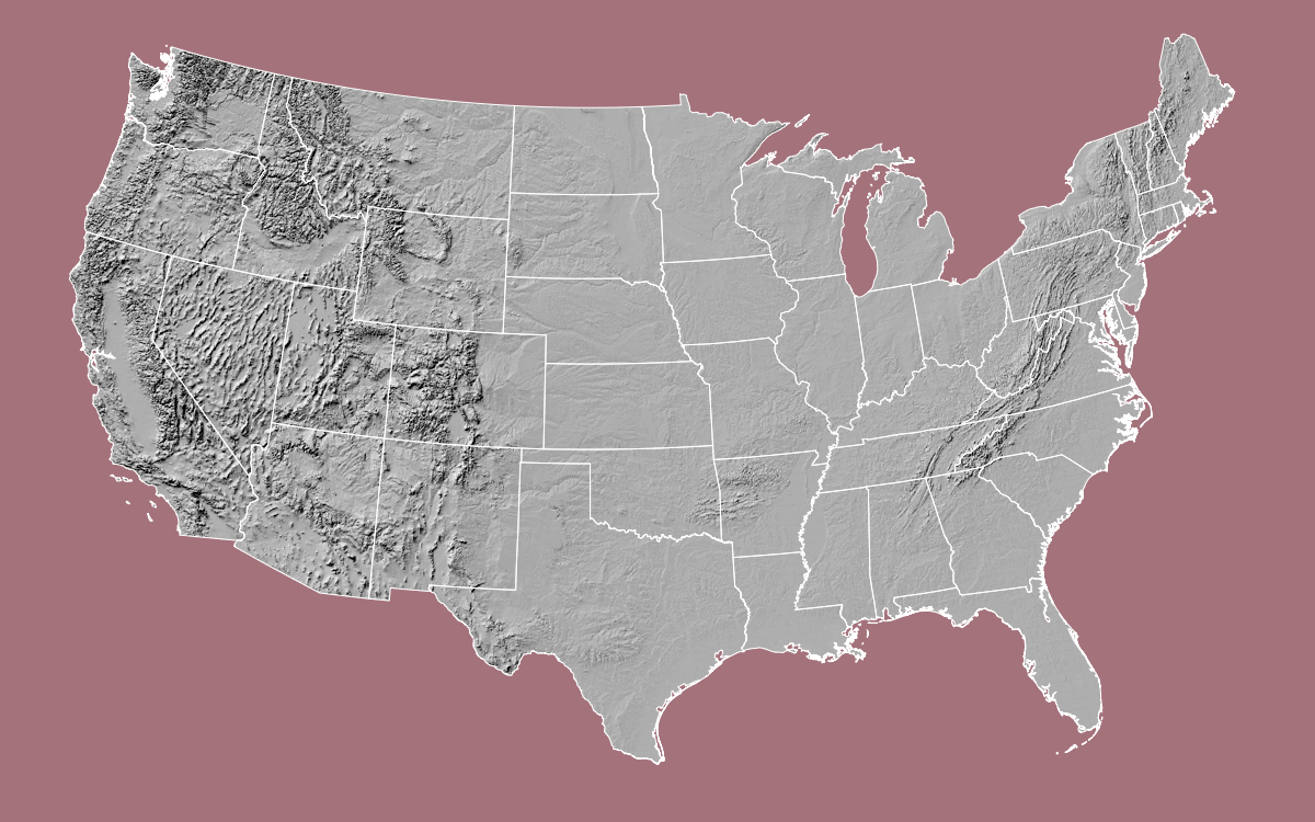
Projections
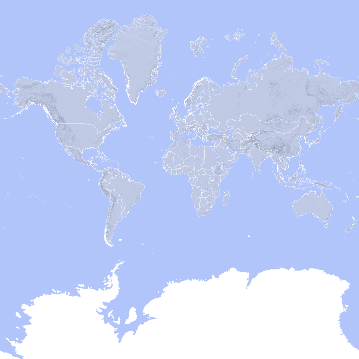
Projections
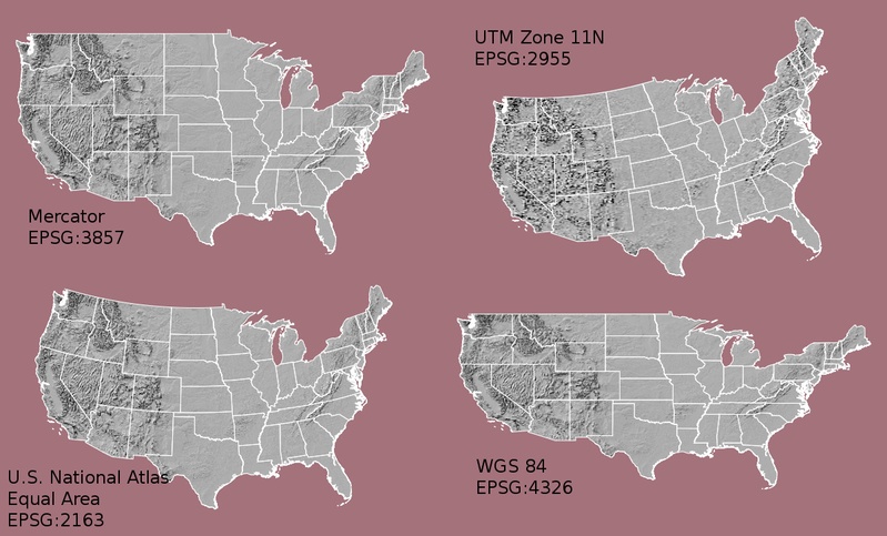
Projections
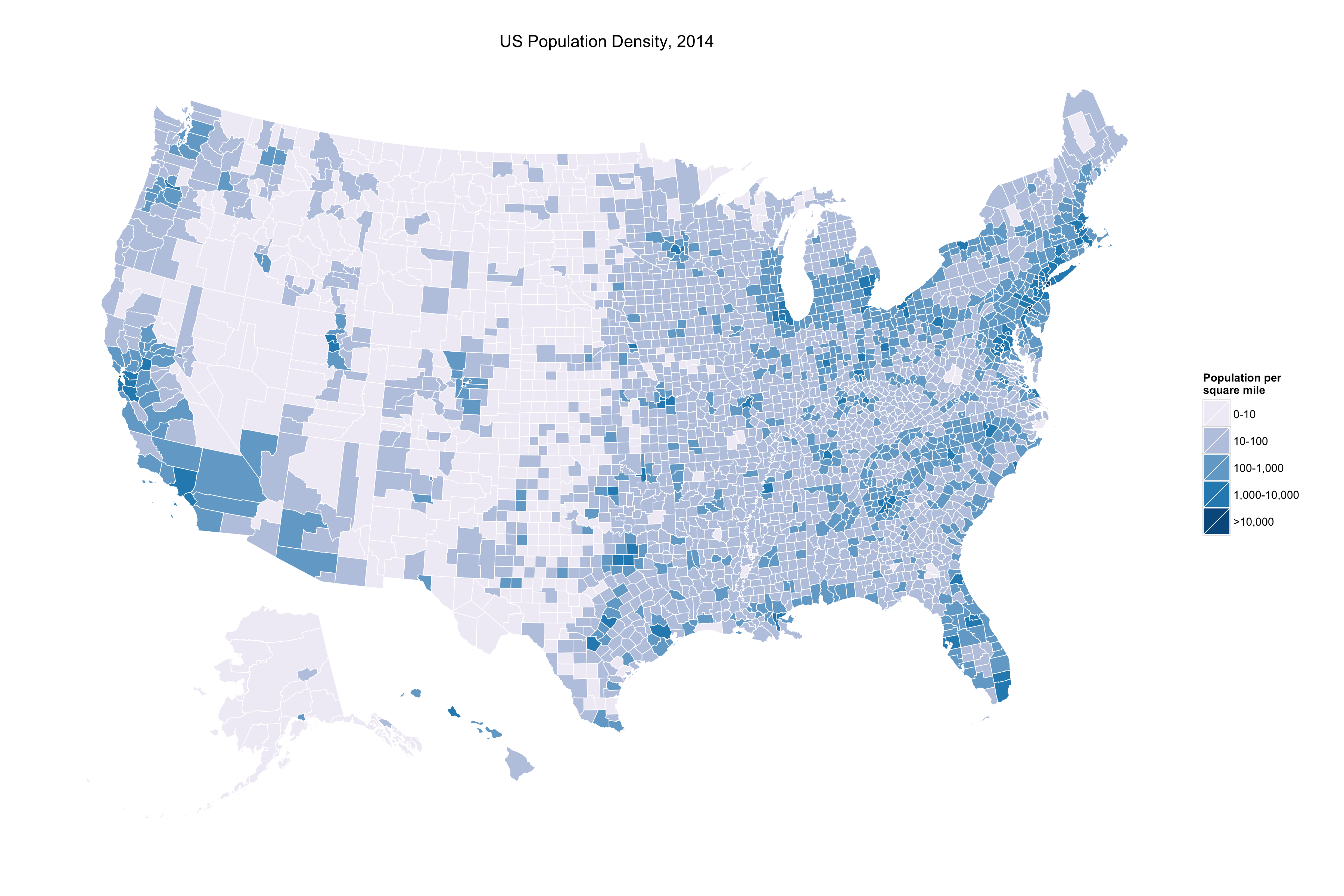
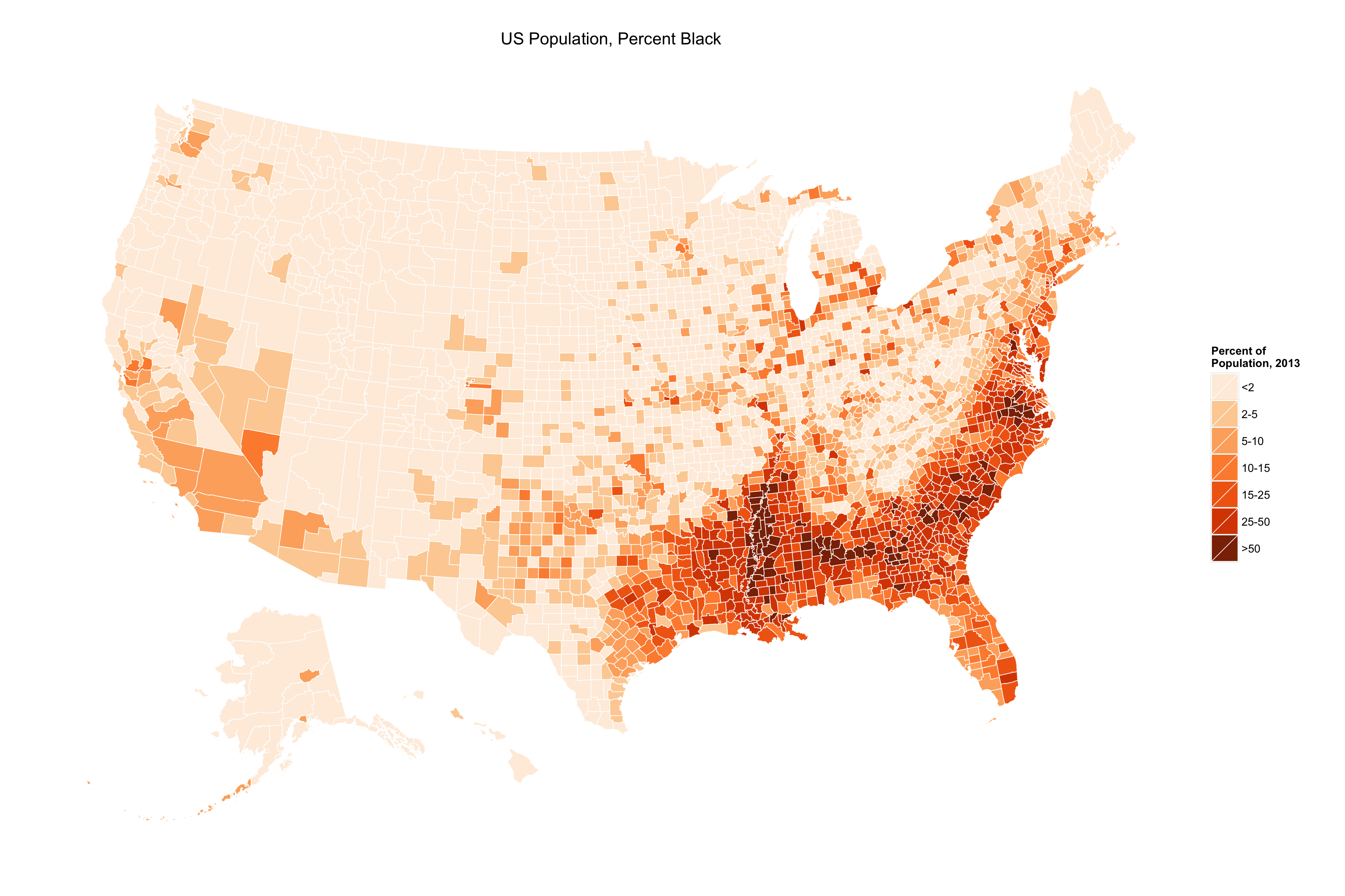
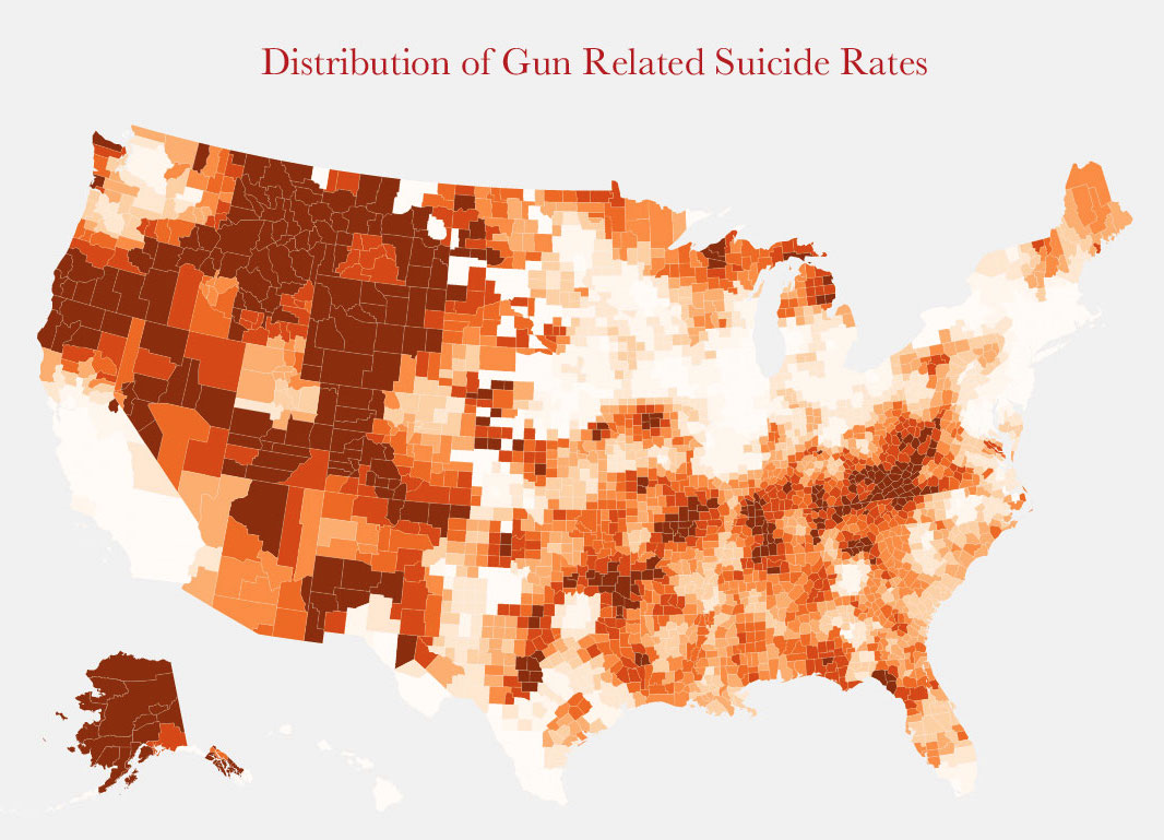
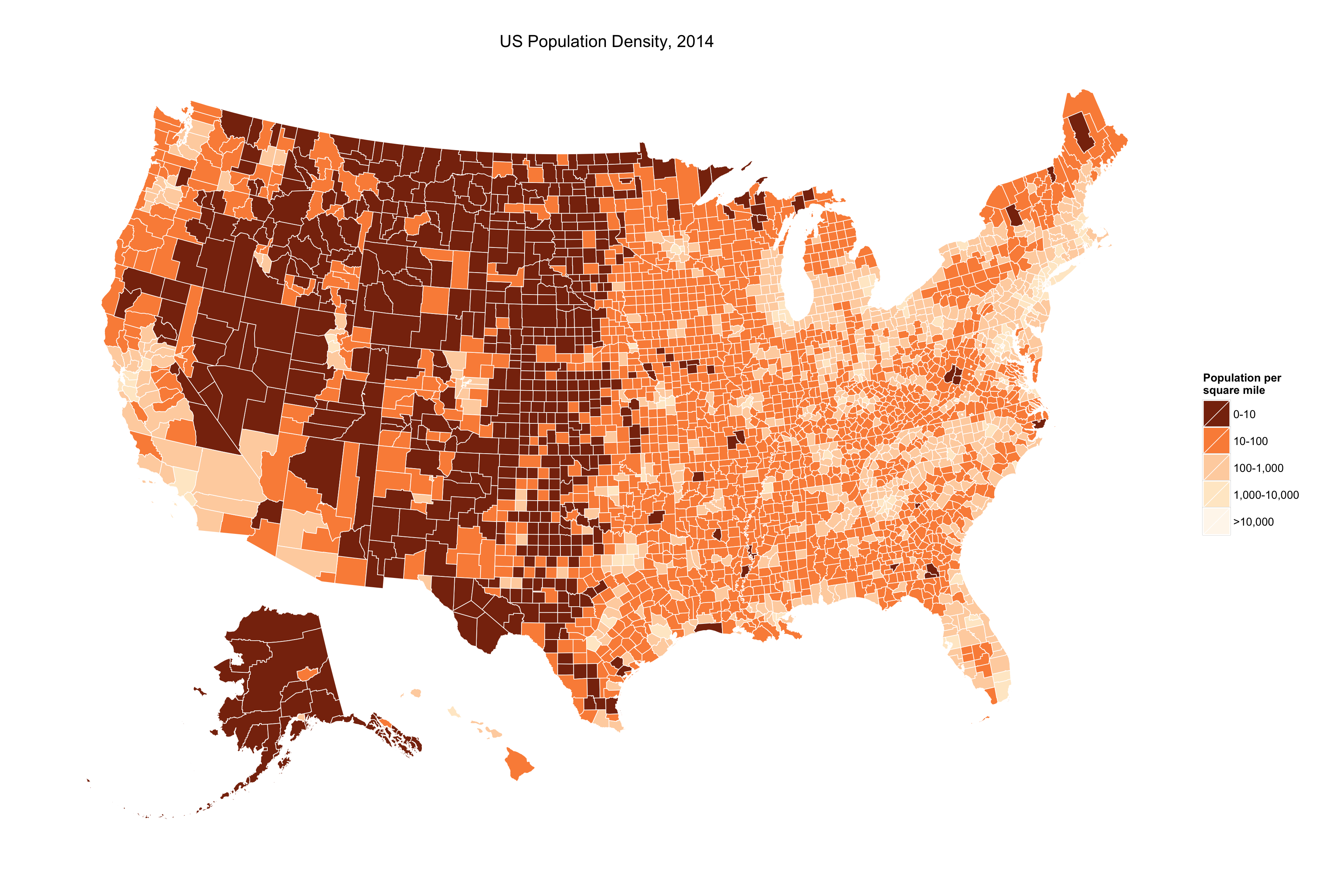
America's Ur-Choropleths
Often, you don't need a 'real' map
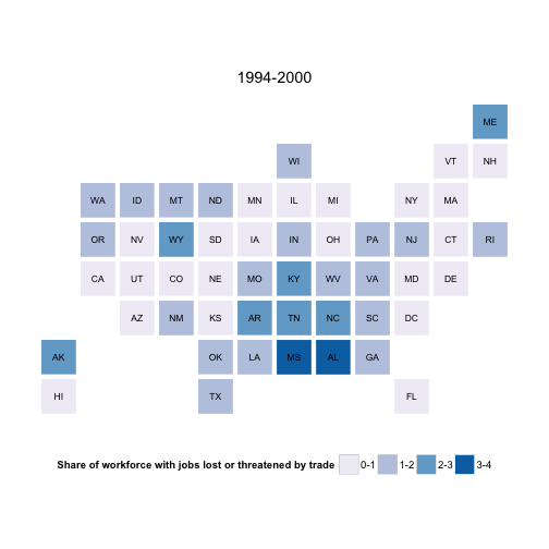
Statebins, by Bob Rudis
devtools::install_github("hrbrmstr/statebins")
## Downloading GitHub repo hrbrmstr/statebins@master
## Installing statebins
## '/Library/Frameworks/R.framework/Resources/bin/R' --no-site-file  \
##   --no-environ --no-save --no-restore CMD INSTALL  \
##   '/private/var/folders/0c/hc2fp3hn3sl1r1pv973q5dsc0000gn/T/Rtmp6batHh/devtools1459e605ca68e/hrbrmstr-statebins-23d1e11'  \
##   --library='/Users/kjhealy/Library/R/library' --install-tests
##
## Reloading installed statebins
dat <- read.csv("http://www.washingtonpost.com/wp-srv/special/business/states-most-threatened-by-trade/states.csv?cache=1", stringsAsFactors=FALSE)
head(dat)
##   fipst stab          state workers1994 workers1995 workers1996
## 1    37   NC North Carolina        3831        2631        8716
## 2     1   AL        Alabama        1504        3527        7627
## 3    28   MS    Mississippi        1613        3344        4454
## 4     5   AR       Arkansas        1376        1107        1473
## 5    47   TN      Tennessee        3210        4149        7297
## 6    45   SC South Carolina        1991        1289        3422
##   workers1997 workers1998 workers1999 workers2000 workers2001 workers2002
## 1       12324        9428       12414        4790       12596       19564
## 2        6858        5340        8697        3919        4400        9895
## 3        1938        3108        6143        2839        3292        4796
## 4        2426        2559        2653         604        3041        3741
## 5        7544        7435        5706        5107        7104        8137
## 6         975        3922        1739        2427        6296        6585
##   workers2003 workers2004 workers2005 workers2006 workers2007 workers2008
## 1       21126       11435       13167       10602       14815       11767
## 2        3285        3156        1895        5358        4156        6377
## 3        3785        1350        1345        1807        2246        3366
## 4        3417        1093        2223        3781        4905        3220
## 5        7528        2673        6156        4849        8254        7262
## 6        5690        4623        5913        5270        3473        4479
##   workers2009 workers2010 workers2011 workers2012 workers2013
## 1       11533       12746        4120        2953        3301
## 2        6661        5306         571        1033         834
## 3        3262         473          77         386         226
## 4        2891        3088        2239        3769         507
## 5        7647        7938        7100        2108        2606
## 6        5846        2575        1513        1864        1321
##   share_cut1994 share_cut1995 share_cut1996 share_cut1997 share_cut1998
## 1           1.4           0.9           3.0           4.1           3.0
## 2           1.1           2.4           5.2           4.6           3.5
## 3           2.0           3.9           5.1           2.2           3.4
## 4           1.6           1.3           1.6           2.7           2.7
## 5           1.6           2.0           3.4           3.5           3.3
## 6           1.5           1.0           2.5           0.7           2.7
##   share_cut1999 share_cut2000 share_cut2001 share_cut2002 share_cut2003
## 1           3.9           1.5           3.8           6.1           6.7
## 2           5.6           2.5           2.8           6.5           2.2
## 3           6.7           3.1           3.6           5.4           4.3
## 4           2.8           0.6           3.1           3.9           3.6
## 5           2.5           2.2           3.1           3.6           3.3
## 6           1.2           1.6           4.1           4.5           3.9
##   share_cut2004 share_cut2005 share_cut2006 share_cut2007 share_cut2008
## 1           3.6           4.1           3.2           4.3           3.4
## 2           2.1           1.2           3.3           2.6           3.9
## 3           1.5           1.5           2.0           2.5           3.7
## 4           1.1           2.3           3.8           4.9           3.2
## 5           1.2           2.7           2.1           3.5           3.0
## 6           3.1           3.9           3.4           2.2           2.8
##   share_cut2009 share_cut2010 share_cut2011 share_cut2012 share_cut2013
## 1           3.5           4.1           1.3           0.9           1.0
## 2           4.3           3.6           0.4           0.7           0.6
## 3           3.7           0.6           0.1           0.5           0.3
## 4           3.0           3.3           2.4           3.9           0.5
## 5           3.4           3.7           3.2           0.9           1.1
## 6           3.9           1.8           1.0           1.2           0.9
##   avgshare avgshare94_00 avgshare01_07 avgshare08_12
## 1     3.56          2.53          4.56          2.64
## 2     3.22          3.55          2.95          2.58
## 3     2.94          3.77          2.99          1.71
## 4     2.89          1.91          3.27          3.16
## 5     2.86          2.64          2.77          2.85
## 6     2.61          1.60          3.57          2.14
p <- statebins(dat, "state", "avgshare94_00", breaks=4,
                labels=c("0-1", "1-2", "2-3", "3-4"),
                legend_title="Share of workforce with jobs lost or threatened by trade",
                font_size=3)

p + theme(legend.position="bottom") +
    ggtitle("1994-2000")
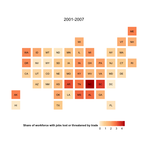
p <- statebins_continuous(dat, "state", "avgshare01_07",
               legend_title="Share of workforce with jobs lost or threatened by trade",
               brewer_pal = "OrRd",
                font_size=3)

p + theme(legend.position="bottom") +
    ggtitle("2001-2007")
library(httr)
library(dplyr)

election_2012 <- GET("https://raw.githubusercontent.com/hrbrmstr/statebins/master/tmp/election2012.csv")

results <- read.csv(textConnection(content(election_2012, as="text")),
                    header=TRUE, stringsAsFactors=FALSE)

results <- results %>%
    mutate(color=ifelse(is.na(Obama), "#2166ac", "#b2182b")) %>%
    select(state, color)
head(results, 15)
##    state   color
## 1     AL #2166ac
## 2     AK #2166ac
## 3     AZ #2166ac
## 4     AR #2166ac
## 5     CA #b2182b
## 6     CO #b2182b
## 7     CT #b2182b
## 8     DE #b2182b
## 9     DC #b2182b
## 10    FL #b2182b
## 11    GA #2166ac
## 12    HI #b2182b
## 13    ID #2166ac
## 14    IL #b2182b
## 15    IN #2166ac
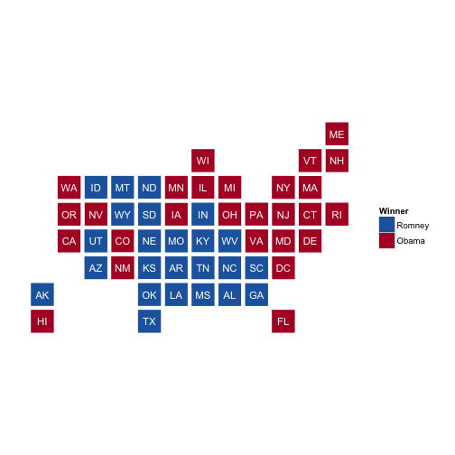
results %>%
    statebins_manual(font_size=4, text_color = "white",
                     labels=c("Romney", "Obama"),
                     legend_position="right",
                     legend_title="Winner")
US County Maps in R
From the Terminal
git clone https://github.com/kjhealy/us-county.git
- Or clone it in your browser, or git client